The Anatomy of our Hopfield Network
An Associative Memory is a dynamical system that is concerned with
the memorization and retrieval of data.
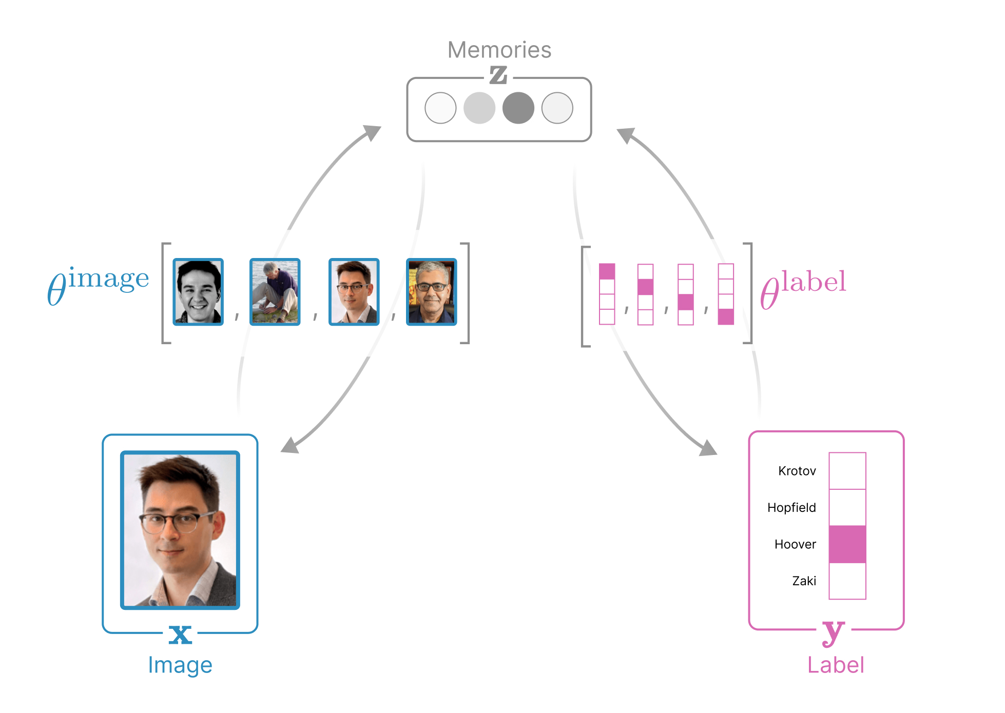
The structure of our data in the demo above is a collection of (image, label)
pairs, where each image variable
x∈R3Npixels is represented
as a rasterized vector of the RGB pixels and each
label variable
y∈RNpeople identifies
a person and is represented as a one-hot vector. Our Associative Memory additionally
introduces a third, hidden variable for the
memories
z∈RNmemories.
In Associative Memories, each of these variables has both an
internal state
that evolves in time and an axonal state
(an isomorphic function of the internal state)
that influences how the rest of the network evolves. This terminology of
internal/axonal is inspired by biology, where the "internal" state is analogous
to the internal current of a neuron
(other neurons don't see the inside of other neurons)
and the "axonal" state is analagous to a neuron's firing rate
(a neuron's axonal output is how it signals to other neurons). We denote the internal state of a variable with a hat: (i.e.,
variable x has internal state x^, y has internal state y^, and z has internal state z^).
Dynamic variables in Associative Memories have two states: an internal
state and an axonal state.
We call the axonal state the activations and they are uniquely
defined by our choice of a scalar and convex Lagrangian function on that
variable
(see Krotov (2021),
Krotov & Hopfield (2021), and Hoover et al. (2022) for
more details). Specifically, in this demo we choose
Lx(x^)≜Ly(y^)≜Lz(z^)≜21i∑x^i2logk∑exp(y^k)β1logμ∑exp(βz^μ)
These Lagrangians dictate the axonal states (activations)
of each variable.
xyz=∇x^Lx=x^=∇y^Ly=softmax(y^)=∇z^Lz=softmax(βz^)
The Legendre transform of the Lagrangian defines the energy of each variable.
ExEyEz=i∑x^ixi−Lx=k∑y^kyk−Ly=μ∑z^μzμ−Lz
All variables in Associative Memories have a special Lagrangian function
that defines the axonal state and the energy of that variable.
In the above equations, β>0 is an inverse
temperature that controls the "spikiness" of the energy function around each
memory
(the spikier the energy landscape, the more memories can be stored). Each of these three variables is dynamic
(evolves in time).
The convexity of the Lagrangians ensures that the dynamics of our
network will converge to a fixed point.
How each variable evolves is dictated by that variable's contribution to
the global energy function
Eθ(x,y,z)
(parameterized by weights θ)
that is LOW when the image
x, the label y, and
the memories z are aligned
(look like real data)
and HIGH everywhere else
(thus, our energy function places real-looking data at local energy minima). In this demo we choose an energy function that allows us to manually
insert memories
(the (image,label) pairs we want to show)
into the weights θ={θimage∈RNmemories×3Npixels,θlabel∈RNmemories×Npeople}. As before, let μ={1,…,Nmemories},
i={1,…,3Npixels} and k={1,…,Npeople}. The global energy function in this demo is
Eθ(x,y,z)=Ex+Ey+Ez+21[μ∑zμ(i∑θμiimage−xi)2−21i∑xi2]−λμ∑k∑zμθμklabelyk=Ex+Ey+Ez+Exz+Eyz
We introduce λ>1 to encourage the dynamics
to align with the label.
Associative Memories can always be visualized as an undirected graph.
Every associative memory can be understood as an undirected graph where nodes
represent dynamic variables and edges capture the
(often learnable) alignment between dynamic
variables. Notice that there are five energy terms in this global energy
function: one for each node
(Ex, Ey, Ez), and one for each edge
(Exz captures the alignment between memories
and our image and Eyz captures the alignment
between memories and our label). See the diagram below for the anatomy of this network.
In fact, every associative memory can be understood as an undirected
graph where nodes
represent dynamic variables and edges capture the
(often learnable) alignment between dynamic
variables. In our energy function, we have three nodes and two edges:
- Image node x representing
the state of our image
- Label node y representing
the state of our label
- Hidden node z representing
the memories
- Edge (x,z) capturing the alignment
of the presented image to our memories
- Edge (y,z) capturing the alignment
of the presented label to our memories
where β>0 is an inverse temperature that
controls the "spikiness" of the energy function around each memory
(the spikier the energy landscape, the more memories can be stored)
and we introduce λ>1 to encourage the
dynamics to align with the label. We use L2 similarity
L2(a,b)=−j∑(aj−bj)2
to capture the alignment of images to the memories stored in
θimage and cosine similarity
cossim(a,b)=j∑ajbj (where ∣∣a∣∣1=∣∣b∣∣1=1)
to capture the alignment of labels to memories stored in θlabel.
It is actually convenient to define a third dynamic variable zμ≜−i∑(θμiimage−xi)2+λk∑θμklabelyk that captures the similarity of (x,y) to the
μth memory
(zμ is dynamic in the sense that it evolves
in time as a function of
x and y). This allows us to reduce visual clutter of the energy function to
This global energy function Eθ(x,y,z) turns
our images, labels, and memories into dynamic variables whose internal states
evolve according to the following differential equations:
τxdtdx^iτydtdy^kτzdtdz^μ=−∂xi∂Eθ=μ∑zμ(θμiimage−xi)=−∂yk∂Eθ=λμ∑zμθμklabel−y^k=−∂zμ∂Eθ=−21i∑(θμiimage−xi)2+λk∑θμklabelyk−z^μ
where τx,τy,τz define how quickly
the states evolve.
The variables in Associative Memories always seek to minimize their
contribution to a global energy function.
Note that in the demo we treat our network as an
image generator
by clamping the labels
(forcing dtdy^=0). We could similarly use the same Associative Memory as a
classifier
by clamping the image
(forcing dtdx^=0) and allowing only the label to evolve.